


Abstract
Nano Co3O4 has been fabricated by co-precipitation of 0.1 M cobalt chloride with 0.1 M oxalic acid. During precipitation, high-frequency signal (9 V) was applied to the precipitation bath. Three samples were prepared at three different frequencies (0 Hz, 400 KHz, 1 MHz). The samples were dried at 120 °C for 20 h, and then calcined at 700 °C for 5 h to obtain the nano Co3O4. The prepared samples were investigated via XRD and TEM studies. According to the present data the particle size decreases from about 164 to 80 nm and the width of the particle size distribution decreases to half of its value with increasing frequency from 0 Hz to 1 MHz.
Export citation and abstract BibTeX RIS

Original content from this work may be used under the terms of the Creative Commons Attribution 3.0 licence. Any further distribution of this work must maintain attribution to the author(s) and the title of the work, journal citation and DOI.
1. Introduction
Nanotechnology has become one of the most important branches of science since the end of the last century. Considerable effort has been made to prepare and characterize nano materials. Nano materials have become attractive because of their unique characteristics that can hardly be obtained from conventional bulk materials. Several physical and chemical processes for synthesis of nanomaterials have been discussed in the literature, including ball milling and annealing [1], arc discharge [2], laser ablation [3–6], chemical vapor deposition (CVD) [7–9], sonochemical method [10], sol-gel technique [11], one-step solid state reaction at room temperature [12], electrochemical [13], thermal decomposition of precursors [14], co-implantation of metal and oxygen ions [15], ultrasonic spray pyrolysis [16], fungus used for producing nanometals [17] and co-precipitation[18–20]. The latter involves preparation of two water solutions: oxalic acid and metal chlorides or oxychlorides. The two solutions interact and precipitate the corresponding metal oxalate in water. During precipitation the solution is subjected to ultrasonic, mechanical or magnetic stirring in order to inhibit crystal growth. The resultant precipitated oxalate is then washed away and calcined to obtain nano oxide powder.
Based on the co-precipitation method described above we suggest a new method for preparation of nanoparticles using a high frequency electric field applied to the precipitation bath during the co-precipitation process. Interesting results have been obtained, and we found that increasing the frequency of the wave leads to a decrease in the size of precipitated nanoparticles and also a decrease in the width of of particle size distribution.
2. Experimental
The chemicals used were of analytical grade and used without further purification. Oxalic acid (C2H2O4.2H2O) and cobalt chloride (CoCl2.6H2O) with purity 99.5% were dissolved in water separately to a concentration of 0.1 M. The aqueous cobalt chloride solution was put in a 100 ml burette and is allowed to drip in the bath containing the oxalic acid solution. The dripping process was completed in 30 min. High frequency ac (sin wave with amplitude 9 V) was applied to the bath, where two aluminium plates are fixed on the opposite walls as electrodes attached to the poles of the signal generators (figure 1). A high frequency generator (EZ Digital FG-8002 2 MHz Sweep Function Generator) was used in this work. The obtained precipitate was dried for 20 h at 120 °C and then calcined at 700 °C for 5 h. Three samples were prepared at three different frequencies 0 Hz, 400 kHz and 1000 kHz. X-ray diffraction (XRD) was performed for the obtained samples using a Brukur D8 Advance Cu-Kα target with secondary monochromator (λ = 1.5411 nm) powered at 40 kV and 40 mA. A high-resolution transmission electron microscope type JEOL—JEM-2100 was used to determine the size of the obtained particles.

Figure 1. Setup used in the present work.
Download figure:
Standard image High-resolution image3. Results and discussion
Figures 2(a)–(c) represent the x-ray diffraction (XRD) patterns of three studied samples at frequencies of 0 Hz, 400 kHz and 1000 kHz, respectively, whereas table 1 contains XRD data and particle size as obtained by the apparatus.
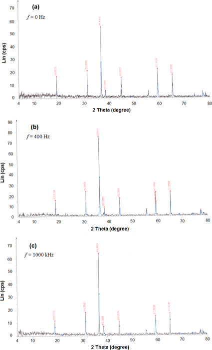
Figure 2. XRD pattern for the samples at different frequencies: (a) 0 Hz, (b) 400 kHz and (c) 1000 kHz.
Download figure:
Standard image High-resolution imageTable 1. Characteristics of three samples at different frequencies 0 Hz, 400 kHz and 1000 kHz.
| Frequency (kHz) | Position | Area | Crystal size (nm) | Microstrain | RMS strain (%) |
|---|---|---|---|---|---|
| 18.93 627 | 2.230 289 | 102.7 | 0.1 | 0.1 | |
| 31.20 333 | 3.295 542 | 149.7 | 0.1 | 0.1 | |
| 36.79 998 | 10.91 055 | 134.7 | 0.1 | 0.1 | |
| 38.50 214 | 1.064 142 | 149 | 0.1 | 0.1 | |
| 0 | 44.7589 | 3.14 245 | 131.1 | 0.1 | 0.1 |
| 55.60 501 | 1.380 412 | 86.3 | 0.1 | 0.1 | |
| 59.29 824 | 5.206 098 | 111.6 | 0.1 | 0.1 | |
| 65.17 876 | 5.393 081 | 94.4 | 0.1 | 0.1 | |
| 400 | 18.95 616 | 2.370 895 | 126.7 | 0.1 | 0.1 |
| 31.22 548 | 4.18 3377 | 134.6 | 0.1 | 0.1 | |
| 36.79 276 | 15.11 863 | 118.3 | 0.1 | 0.1 | |
| 38.52 218 | 1.437 274 | 111.9 | 0.1 | 0.1 | |
| 44.77 339 | 3.481 362 | 136.5 | 0.1 | 0.1 | |
| 55.62 812 | 1.672 278 | 127.7 | 0.1 | 0.1 | |
| 59.30 882 | 5.802 912 | 113.3 | 0.1 | 0.1 | |
| 65.18 947 | 6.038 181 | 115.2 | 0.1 | 0.1 | |
| 1000 | 18.95 383 | 2.340 706 | 66.4 | 0.1 | 0.1 |
| 31.24 691 | 3.595 495 | 110.9 | 0.1 | 0.1 | |
| 36.80 309 | 14.23 802 | 113.3 | 0.1 | 0.1 | |
| 38.50 991 | 1.362 553 | 108 | 0.1 | 0.1 | |
| 44.76 884 | 2.624 825 | 120.4 | 0.1 | 0.1 | |
| 55.5943 | 1.049 637 | 91.8 | 0.1 | 0.1 | |
| 59.30 854 | 4.383 658 | 75.6 | 0.1 | 0.1 | |
| 65.19 451 | 5.771 366 | 85.7 | 0.1 | 0.1 |
Transmission electron microscope (TEM) images of three these studied samples are given in figures 3(a)–(c), respectively.

Figure 3. (a) TEM images for the obtained sample at three different frequencies: (a) 0 Hz, (b) 400 kHz and (c) 1000 kHz.
Download figure:
Standard image High-resolution imageFigures 4 and 5 represent the particle size as measured by the electron microscope and calculated by the x-ray versus signal frequency, respectively. In figure 4, the circles and the squares represent the maximum and minimum particle size seen in the photograph, respectively. Figure 5 shows the particle size corresponding to the maximum peak in the x-ray chart. Figure 6 illustrates the width of the particle size distribution (nm) versus the applied frequency as obtained from figure 4.
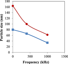
Figure 4. Particle size as measured by TEM versus frequency. Solid circles and solid squares are the highest and the lowest particle size, respectively.
Download figure:
Standard image High-resolution image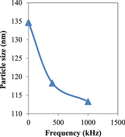
Figure 5. Particle size as measured by XRD versus frequency.
Download figure:
Standard image High-resolution image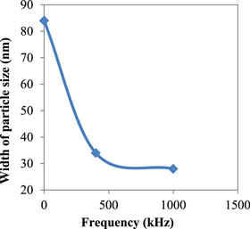
Figure 6. Distributions width of the particle size distributions (nm) versus frequency taken from figure 4.
Download figure:
Standard image High-resolution image
As is clear from figures 4 and 5 the particle size decreases with the increase in frequency of the applied signal, whereas figure 6 shows decreasing width of particle size distribution when frequency is increased from 0–1000 kHz.
Upon subjection to a mechanical or magnetic stirring, circulation motion starts in the bulk of the solution present in the bath, which disturbs the growth of the precipitated crystals. In the case of ultrasonic applications, the volume from the liquid with the dimension of ultrasonic wavelength oscillates and so inhibits the crystal growth. In the case of application of HF, the ions themselves will oscillate such that the positively charged cations follow the electric field while the negatively charged anions will move against the field, preventing the formation of the crystals. It is interesting to note that in both cases represented by squares and circles in figure 4, the particle size and the width of the particle size distribution shrinks to the half of its value at zero frequency.
At higher frequency, the wavelength is shorter and the periodical time is smaller, which means that the cations will follow the field for a smaller time and short distance, regarding that the distribution of the oxalate anions in the solution is homogenous. This will reduce the chance for build-up of the metal oxalate particle. Because of this, in the higher frequency case the particle size is smaller than that of the lower frequency case.
4. Conclusion
A new method is suggested, by which fine tuning of the particle size is possible. More work should be done to formulate the effect of different parameters of the cations, HF wave and the solution normality on the particle size. This will be our future work.