

Abstract
We study the critical behaviour of very thin magnetic films. This system can be described by the q-state clock model. In order to determine the critical exponents of the system when there exists the Berezinskii–Kosterlitz–Thouless phase between the two phase transitions, we introduce a new technique for calculating the order parameter. The simulation is performed by very high-resolution Monte Carlo method with including the Wang–Landau algorithm. The results showed that the Berezinskii–Kosterlitz–Thouless phase starts to occur when  with a small symmetry breaking field. We obtained not only the critical exponents of a common transition at high temperature but also the ones of unclear transition at low temperature.
Export citation and abstract BibTeX RIS

Original content from this work may be used under the terms of the Creative Commons Attribution 3.0 licence. Any further distribution of this work must maintain attribution to the author(s) and the title of the work, journal citation and DOI.
1. Introduction
During the last 40 years, physics of materials of nanometric size have attracted a wide interest. This is due to important applications in industry [1, 2]. An example is the so-called giant magneto-resistance (GMR) used in data storage devices, magnetic sensors... [3–6]. The experimental researches are often immediately used for industrial applications without waiting for a full theoretical understanding. In parallel to these experimental developments, much theoretical effort has also been devoted to the search of physical mechanisms lying behind new properties found in nanoscale objects such as ultrathin films, ultrafine particles, quantum dots, spintronic devices, etc. This effort aimed not only at providing explanations for experimental observations but also at predicting new effects for future experiments [7, 8]. The physics of two-dimensional (2D) systems is very exciting. Some of those 2D systems can be exactly solved: one famous example is the Ising model on the square lattice [9]. In thin films, there is a crossover from 2D to three-dimensional (3D) behavior as the film thickness increases [10]. Another interesting result is the absence of long-range ordering at finite temperatures for the continuous spin models (XY and Heisenberg models) in 2D [11]. In general, 3D systems for any spin models cannot be unfortunately solved. However, several methods in the theory of phase transitions and critical phenomena can be used to calculate the critical behaviors of these systems [12].
One of the most fascinating tasks of statistical physics is the study of the phase transition in systems of interacting particles. In particular, different kinds of transition from one phase to another have been efficiently studied by theory of renormalization group, high–low-temperature expansions [12], exact methods [13], numerical simulations [14], etc. Most phase transitions belong to either the first-order type or the second-order type. Specially, the Kosterlitz–Thouless (KT) transition is observed in superfluid systems which can be described by the 2D XY model [15].
On the other hand, q-state ferromagnetic clock model is a discrete version of the XY model, and is also known as the vector Potts model that consists of 2D planar spins with q different orientations. At the limiting cases, for  , the clock model reduces to the Ising model, while for
  , it is XY-like model. However, for
  , ones believed that a Berezinskii–Kosterlitz–Thouless (BKT) phase should occur between the ferromagnetic phase and the paramagnetic phase [15, 16]. This model is of great interest, because there is a controversy on the number of phase transitions and the character of the phase transitions [17–23]. In this paper we investigate the critical properties of thin magnetic film systems using the q-state clock model. For carrying out this purpose, we shall use Monte Carlo (MC) simulations with highly accurate Wang-Landau algorithm (flat histogram technique) [24]. We introduce a modified definition of the order parameter. Thus, the critical exponents can be determined for the transitions at both low and high temperature.
The paper is organized as follows. Section 2 is devoted to the description of the model and the simulation technique. Section 3 presented the simulation results. Concluding remarks are given in section 4.
2. Model and the simulation technique
We consider the clock model on a thin film made from the ferromagnetic square lattices. The size of the film is  with
with  being the film thickness. The spin is considered as a planar vector of magnitude
  with two components,
  . The Hamiltonian is given by
where the sum  runs over all the nearest-neighbor (NN) pairs.
  (in units of energy) is the ferromagnetic exchange coupling and
  being qth order symmetry-breaking field.
  is the angle of spin
  makes with the x axis.
In order to investigate the nature of the phase transition of this system, we use the standard MC method and the Wang–Landau technique of simulation. Wang and Landau have proposed an MC algorithm for classical statistical models which allowed to study systems with difficultly accessed microscopic states [24]. The algorithm uses a random walk in the energy space to get an accurate estimate for the density of states (DOS)  , which is defined as the number of spin configurations for any given
  . This method is based on the fact that a flat energy histogram
  is produced if the probability for the transition to a state of energy
  is proportional to
  . We summarize how this algorithm is implied here. At the beginning of the simulation, the density of states
  is unknown so all densities are set to unity,
  . We start a random walk in energy space
  by choosing a site randomly and flipping its spin with a transition probability
where  is the energy of the current state and
  is the energy of the proposed new state. Each time an energy level
  is visited, the DOS is modified by a modification factor
  whether the spin is flipped or not, i.e.
  . Initial value of the modification factor
  can be as large as
  . A histogram
  records the number of times a state of energy
  is visited. Each time the energy histogram satisfies a certain 'flatness' criterion, the histogram
  is then reset to zero, and the modification factor is reduced, typically to the square root of the previous factor, to produce a finer estimate of
  . The reduction process of the modification factor
  is repeated several times until a final value
  which is close enough to one. The histogram is considered as flat if

for all energies, where x% is chosen between 90% and 95% and  is the average histogram.
The thermal average of a thermodynamic quantity  can be evaluated by
in which
Thermal averages of physical quantities are thus calculated as continuous functions of T, now the results should be valid over a much wider range of temperature.
In MC simulations, one calculates the magnetic susceptibility defined by
 being the magnetization (also called the order parameter). It has following form:
For the q-state Potts model, the value of spins is taken from a finite set of integers  . Therefore, the order parameter is defined by other equation
with
where  is the number of spins which have a same value
  .
.
In order to study the critical behaviors, we use the scaling relations given by


 and
and  being the critical exponents.
  is nth order cumulant of the order parameter which is written in the form
Here, the order parameter  is replaced by either
  in equation (7) or
  in equation (8). In this paper, we only estimate
  from
from  , with this value we calculate
  from
from  .
.
Let us discuss on a specific case of  , there exists two transitions which separate the system into three phases: ferromagnetic phase, BKT phase and the paramagnetic phase [22]. These phase transitions are characterized by non-universal critical exponents. The system undergoes from ferromagnetic phase to BKT phase passing through the first transition at low temperature (ferromagnetic-BKT transition), and then it passes through the second transition at high temperature (BKT-paramagnetic transition). From the MC simulation results, although the plot of the specific heat clearly showed a peak for the ferromagnetic-BKT transition at low temperature, ones could not estimate the critical exponents
  and
and  because there was no peak in the plots of susceptibility and nth order cumulant. In other words, the definitions of the order parameter (7) and (8) were not usable for calculating the critical exponents of the ferromagnetic-BKT transition at low temperature (the first transition).
Now, we suggest a new method for the calculation of the order parameter by modifying the definition of  in equation (9), i.e.
  is the total number of the spin vectors within ith circular sector
  with central angle
 . The central angle satisfies the condition
  and it is defined by
where  are the angles corresponding to the maximum of anisotropic term in the Hamiltonian (1), i.e.
  or
or  with
with  . Then formula (13) becomes
For example, since the system has four-states ( ), we obtain
3. The simulation results
In this section, we consider a special case of  for comparing with previous results. We shall present the results obtained by MC simulations using the Wang-Landau algorithm. Note that the order parameter is obtained from equations (8), (9) and (14). The xy linear sizes N = 20, 30, ..., 80 have been used in our simulations. Errors shown in the following have been estimated using statistical errors, which are very small and fitting errors given by fitting software.
Let us consider a specific case of  with a strong field
  for testing the new method of the calculations. It is well know that the system becomes 2D Ising-like model in limit
  with a single phase transition. We calculate the universal critical exponents
  and
and  by following the expressions (10)–(12). We show in figures 1 and 2 the maximum of 2nd order cumulant and the maximum of susceptibility versus lattice size in the ln–ln scale, respectively. If we use the equations (10) and (11) to fit these lines, i.e. without correction to scaling, we obtain
  and
and  from the slopes of the remarkably straight lines. For
  , we have
  which yields
  and
and  yielding
  . These results are in excellent agreement with the exact results
  and
and  . Thus, we can conclude that our calculation method is applicable for the clock model. We summarize in table 1 the estimative values of
  and
and  for several values of symmetry-breaking field
  and 0.5. The critical exponents are slightly decrease with increasing
  .
.
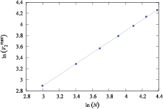
Figure 1. Maximum of V2 versus N in the ln − ln scale.
Download figure:
Standard image High-resolution image
Figure 2. Maximum of susceptibility versus  in the ln − ln scale.
Download figure:
Standard image High-resolution imageTable 1. The critical exponent for  with several
  and 0.5.
 |
 |
 |
 |
 |
|---|---|---|---|---|
| 0.01 | 0.864 99 ± 0.006 | 1.640 55 ± 0.013 | 1.156 08 | 1.896 61 |
| 0.05 | 0.971 01 ± 0.005 | 1.737 89 ± 0.002 | 1.029 86 | 1.789 78 |
| 0.10 | 0.991 63 ± 0.006 | 1.734 76 ± 0.008 | 1.008 44 | 1.749 40 |
| 0.50 | 1.005 66 ± 0.003 | 1.749 01 ± 0.006 | 0.994 37 | 1.739 17 |
For  , there is still a single transition at high temperature. If
  , the critical exponents are most likely to that of Ising-like case. As see in table 2, the critical exponents have an unusual value for
  . This transition is mixed of the two transitions: ferromagnetic-BKT transition and BKT-paramagnetic transition. It indicates that the BKT phase starts to occur from
  with
with  is small enough.
Table 2. The critical exponent for  with several
  and 0.1.
 |
 |
 |
 |
 |
|---|---|---|---|---|
| 0.01 | 0.604 46 ± 0.003 | 1.149 02 ± 0.018 | 1.654 37 | 1.900 90 |
| 0.03 | 0.656 67 ± 0.002 | 1.793 59 ± 0.020 | 1.522 83 | 2.731 34 |
| 0.05 | 0.699 56 ± 0.004 | 1.774 09 ± 0.020 | 1.429 47 | 2.536 01 |
| 0.10 | 0.852 91 ± 0.018 | 1.860 17 ± 0.013 | 1.172 46 | 2.180 97 |
For  and
and  , we show in figure 3 the peak of the susceptibilities located around the critical temperature
  . This is the second transition at high temperature (BKT-paramagnetic transition). The maximum of susceptibility increases with increasing the system size that is a signature of the phase transition. Note that, the susceptibilities
  are obtained by using equations (6) and (7). Therefore, our result is in good agreement with the previous result (see figure 1 in [22]). Besides, the curves of
  have a prominence located around
  which is expected to be the first transition at low temperature (ferromagnetic-BKT transition). Of course, ones could not obtain the critical exponents of this transition because there is no peak in the plots of the susceptibility and the second order cumulant. In contrast, if the set of equations (6), (8), (9) and (14) are applied for calculating the magnetization, then we can obtain the expected susceptibilities which are presented in figure 4. It clearly shows two peaks corresponding to the two transitions: one is BKT-paramagnetic transition at high temperature
  and the other one is the ferromagnetic-BKT transition at low temperature
  . The critical exponents
  and
and  are given in tables 3 and 4 for the first and the second phase transition, respectively. These results are again in good agreement with the experimental data [23].

Figure 3. Susceptibility  versus temperature for several lattice sizes, with
  and
and  .
.
Download figure:
Standard image High-resolution image
Figure 4. Susceptibility versus temperature for several lattice sizes, with  and
and  .
.
Download figure:
Standard image High-resolution image
Table 3. The critical exponent of the ferromagnetic-BKT transition with  and several
  and 0.5.
 |
 |
 |
 |
 |
|---|---|---|---|---|
| 0.01 | 0.481 76 ± 0.008 | 1.115 49 ± 0.017 | 2.075 72 | 2.315 44 |
| 0.05 | 0.524 28 ± 0.006 | 1.316 56 ± 0.021 | 1.907 37 | 2.511 17 |
| 0.10 | 0.581 61 ± 0.007 | 1.389 87 ± 0.015 | 1.719 36 | 2.389 69 |
| 0.50 | 0.647 42 ± 0.005 | 1.531 46 ± 0.006 | 1.518 65 | 2.365 48 |
Table 4. The critical exponent of the BKT-paramagnetic transition with  and several
  and 0.5.
 |
 |
 |
 |
 |
|---|---|---|---|---|
| 0.01 | 0.599 74 ± 0.007 | 1.607 60 ± 0.011 | 1.667 39 | 2.680 49 |
| 0.05 | 0.588 63 ± 0.009 | 1.607 78 ± 0.011 | 1.698 86 | 2.731 39 |
| 0.10 | 0.593 90 ± 0.009 | 1.604 07 ± 0.010 | 1.683 79 | 2.700 91 |
| 0.50 | 0.658 48 ± 0.006 | 1.529 24 ± 0.008 | 1.518 65 | 2.322 38 |
Before closing this section, let us discuss on the behavior of the phase transition for  . The critical exponents do not depend neither on the number of state nor symmetry-breaking field. From the simulation results, we obtain the critical exponents
  and
and  for the first transition,
  and
and  for the second transition.
4. Concluding remarks
We have studied a system, namely the q-state clock model on the thin film. The order parameter was calculated by using the new definitions. Therefore, we could easily determine the maxima of the susceptibility and nth order cumulant of order parameter, though the system size was very small. For the simulations, we considered the 2D case in order to clarify the point whether or not there was an existence of the BKT phase with varying q state and hq field.
From the results obtained by very highly accurate flat histogram technique shown above, we conclude that the existence of the BKT phase strongly depends on both q and hq. In the case q = 3, the BKT phase starts to occur when  . While it starts to occur when
  for q = 4. Note that, this phase is always observed for the five-state and six-state [17].
For the BKT-paramagnetic transition at high temperature, the critical exponents slightly change with varying q state and hq due to the statistical errors. For the first transition at low temperature (ferromagnetic-BKT transition), the non-universal critical exponents strongly depend on hq when q < 5 while these have a few changes if otherwise. Our results confirmed the validation of the previous expectation [22] and the experimental data [23].
Acknowledgment
This work was supported by the NAFOSTED (National Foundation for Science and Technology Development, Vietnam), Grant No. 103.02–2011.55.